Multiple imputation

In multiple imputation, the imputatin process is repeated multiple times resulting in multiple imputed datasets. In this method the imputation uncertainty is accounted for by creating these multiple datasets. The multiple imputation process contains three phases: the imputation phase, the analysis phase and the pooling phase (Rubin, 1987; Shafer, 1997;  Van Buuren, 2012). 

Multiple imputation works well when missing data are MAR (Eekhout et al., 2013). In the imputation model, the variables that are related to missingness, can be included. That way bias is reduced and estimates are more precise. 

In the first phase, the imputation phase, several copies of the data set are created each containing different imputed values. The imputed values are estimated using the means and covariance of the observed data. Regression equations are used to predict the incomplete values from the complete values and a normally distributed residual term is added to each value to restore variability. This procedure is similar to stochastic regression imputation. This process is iterated several times, updating the regression parameters after every iteration, to obtain different imputed values each time. Every so many iterations, one imputed dataset is stored until the required number of imputed datasets is reached.

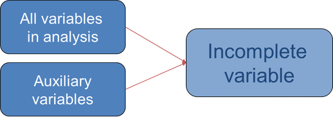
The specification of the correct imputation model is very important for the performance of multiple imputation. Firstly, it is important to include the correct variables in the imputation process. Accordingly, all variables that are of substantial interest should be included in the imputation model, so the predictor variables, covariates and outcome variables from the main analysis. Besides these variables, auxiliary variables can be included to improve the estimation of the imputed values. The figure below displays the content of an imputation model. Secondly, it is important to have an imputation model that fits the distribution assumptions of the data. So when incomplete data are continuous and normally distributed, a multivariate normal distribution or linear regression can be used for the imputation. However, when data are not normal, or not continuous other imputation algorithms should be applied.

In the second phase, the analysis phase, the statistical analysis is carried out. On each imputed dataset, the analysis is carried out that would have been applied had the data been complete. That way as many sets of results are created as the number of imputed datasets created in the imputation phase. 

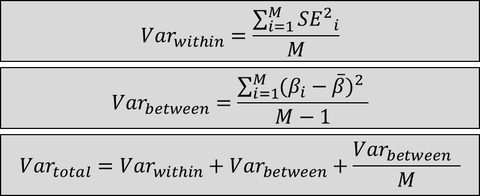
Finally, in the pooling phase, the multiple sets of results or parameter estimates are combined into a single set of results. When the estimates are pooled by Rubin's Rules, the parameter estimates are summarized by taking the average over the parameter estimates from all imputed datasets. The standard errors are pooled by combining the within imputation variance and the between imputation variance. The formulas for this procedure are depicted in the figure below.